‘If intelligence was a cake, unsupervised learning would be the cake, supervised learning would be the icing, and reinforcement learning would be the cherry on top’
In other words, there is a huge potential in unsupervised learning.
One form or unsupervised learning is grouping similar instances together in clusters. Clustering is a great tool for data analysis, customer segmentation, recommendation systems, search engines, semi-supervised learning, dimensionality reduction and more.
If you wander around a park on your one lockdown walk a day, you may stumble upon a tree you have never seen before. If you look around and notice a few more, which are not identical but are similar enough looking that you know they belong to the same genus. You may need an arborist to tell you which species it is, but you don’t need the expert to just group your trees into similar looking groups. This is the essence of clustering: the task of identifying similar instances, and assigning them into clusters, or groups of similar instances.
K-Means
One of the most commonly used clustering techniques is K-means. The K-means algorithm was proposed by Stuart Lloyd and Bell Labs in 1957 as a technique for pulse-code modulation, but only published outside the company in 1982. Edward Forgy published virtually the same algorithm in 1965 so it is referred to as Lloyd-Forgy. The following generates our data which we will cluster:
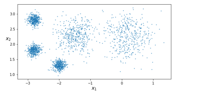
from sklearn.datasets import make_blobsblob_centers = np.array([[ 0.2,  2.3],[-1.5 ,  2.3],[-2.8,  1.8],[-2.8,  2.8],[-2.8,  1.3]])blob_std = np.array([0.4, 0.3, 0.1, 0.1, 0.1])X, y = make_blobs(n_samples=2000, centers=blob_centers,
cluster_std=blob_std, random_state=7)plt.figure(figsize=(8, 4))
plot_clusters(X)
save_fig("blobs_plot")
plt.show()

K-Means is very efficient at clustering data like the set above, often in very few iterations. It will try to find the centre of each cluster, and assign each instance to the closes cluster. Let’s train a K-Means cluster:
from sklearn.cluster import KMeans
k = 5
kmeans = KMeans(n_clusters = k)
y_pred = kmeans.fit_predict(X)
Each instance is assigned to one of the five clusters. It receives a label as the index of the cluster it gets assigned to.
We can see these labels:
y_pred
array([4, 0, 1, ..., 2, 1, 0], dtype=int32)y_pred is kmeans.labels_
True
We can also see the five centroids (cluster centres) that the algorithm found:
kmeans.cluster_centers_
array([[ 0.20876306,  2.25551336],
       [-2.80580621,  1.80056812],
       [-1.46046922,  2.30278886],
       [-2.79290307,  2.79641063],
       [-1.99213367,  1.3131094 ]])
We can easily do this for new data too, by seeing which centroid any new data point is closest to. We can also visualise the decision boundaries, and each centroid is represented by X.

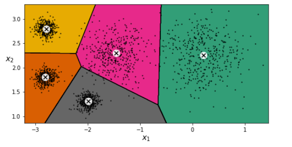
Initially, centroids are placed randomly, instances labelled, and the centroids are updated. This process iterates until the centroids stop moving, and the clusters have been defined.
Accelerated K-Means
Accelerated K-Means is the default for Sklearn. it considerably accelerates this algorithm by keeping track of the lower and upper bounds for the distances between instances and centroids. You can force Sklearn to use the original algorithm, although its unlikely to be needed.
Mini-batch K-Means
Instead of using the full dataset at each iteration, the algorithm is capable of using mini-batches, moving the centroid slightly at each iteration. This increases the speed of the algorithm by a factor of 3–4 typically. Especially important, it makes it possible to cluster huge datasets that do not fit in memory. One limitation is that its inertia is usually slightly worse, especially as clusters increase, however with many clusters the speed is much faster using mini-batch.
Finding the optimal number of clusters
In this dataset we can see that there are clearly 5 clusters we want to segment from each other. However that is not always the case, and often our data isn’t as obviously segmented as this. Our result can be quite poor if we don’t take precautions to figure out the optimal number of clusters:

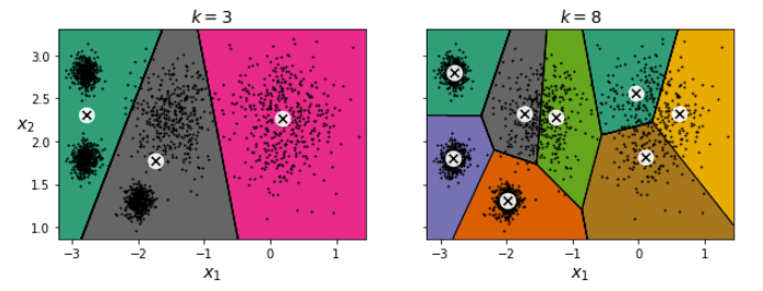
The first thought is to choose the k which minimises inertia, however we cannot do that as inertia will always decrease with a higher k. Indeed, the more clusters there are, the closer each instance will be to its closest centroid, and therefore the lower the inertia will be. As we can see with a k=8, we are splitting clusters for no good reason.

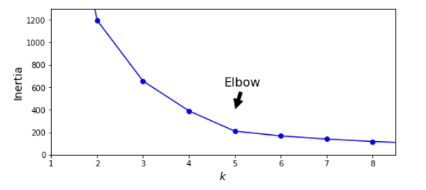
Inertia drops very quickly up to 5, but then it decreases very slowly afterwards. Any k lower than 5and the gain would be dramatic, and any higher and we are not gaining much more information. This is a rather rough, subjective way of assigning k, however it generally works pretty well. When doing this it allows us to take context of a specific needs of a business problem too.
However, in this case we could see that there were 5 clusters we wanted to segment. 4 clusters may be adequate but we should investigate the difference between k=4 and k=5
Silhouette Score
Another, more precise approach is to use silhouette score for each instance and plot them for different numbers of clusters, however it is more computationally intensive, it will give us a more clear optimal k:
from sklearn.metrics import silhouette_scoresilhouette_score(X, kmeans.labels_)silhouette_scores = [silhouette_score(X, model.labels_) for model in kmeans_per_k[1:]]

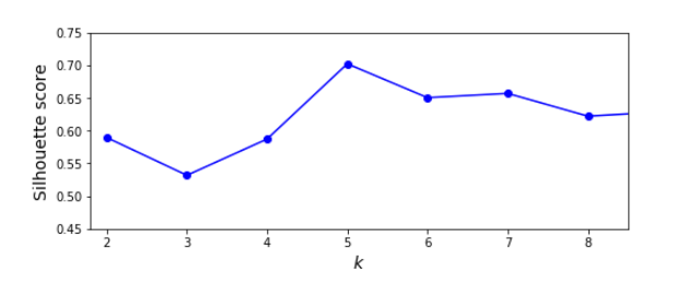
As we can see, using silhouette score for each level of k, it is far more obvious which k is optimal.
Even more informative is plotting every instances silhouette coefficient, sorted by the cluster they are in and by the value of the coefficient. This is a silhouette diagram. The shapes height indicates number of instances the cluster contains, and its width represents the sorted silhouette coefficients of the instances in the cluster (the wider the better). The dashed line indicates the mean silhouette coefficient.

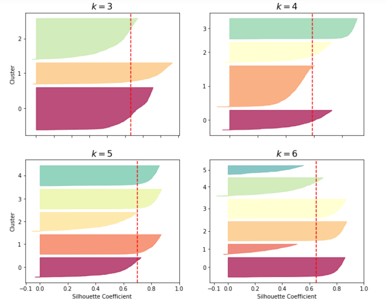
The vertical dashed lines represent the silhouette score for each number of clusters. If many instances stop short (left) of the dashed line, then the cluster is rather bad because it means the instances are much too close to each other. at k=3, and k=6 we get bad clusters, but at k=4 and k=5 they are pretty good. Most instances extend beyond the dashed line. When k=4 though, the orange cluster is rather big, and at k=5 they are all similar sizes, so it seems like 5 should be used to get clusters of similar sizes.
Performing this process shows a clear limitation of the elbow method, and doing it regularly can reinforce the robustness of your choices of k.
K-Means Limitations
To be a good data scientist, it’s important to know the assumptions behind methods you use so that you have an idea about the strength and weakness of them. This will help you decide when to use each method and under what circumstances:
- Often we can end up with suboptimal solutions and a local minima (due to the random initialisation of centroids), so it’s important to run the algorithm several times to avoid this.
- As well as this, we need to specify k, which can be subjective and quite a hassle sometimes, depending on the dataset.
- And the largest problem is that K-Means does not perform particularly well when clusters are different sizes, densities or non-spherical shapes. Depending on the data, another clustering algorithm may work better. (Often, scaling input features before performing K-Means can help with this, however it does not guarantee all clusters will be nice and spherical)
- K-Means also gives more weight to bigger clusters than smaller ones. In other words, data points in smaller clusters may be left away from the centroid in order to focus more on the larger cluster. This can lead to poorly assigned smaller clusters simply because of unbalanced data.
- And finally, because K-Means assigns each instance into a non-overlapping cluster, there is no measure of uncertainty for points that lie near boundary lines
In this article, I discussed one of the most famous clustering algorithms — K-Means. We looked at the challenges which we might face while working with K-Means.
We implemented k-means and looked at the elbow curve which helps to find the optimum number of clusters in the K-Means algorithm, and showed its limitations too.
If you have any doubts or feedback, feel free to share them in the comments section below
References
Aurelien Geron (2019) Hands-On Machine Learning with Scikit-Learn, Keras, and TensorFlow: Concepts, Tools, and Techniques to Build Intelligent Systems Book , 2 edn., : O’Reilly.
No comments:
Post a Comment