Understanding the concept of Hierarchical clustering Technique

 Hierarchical clustering Technique:

Hierarchical clustering is one of the popular and easy to understand clustering technique. This clustering technique is divided into two types:

1. Agglomerative
2. Divisive

Click Here To Claim Yout Complimentary McDonald’s Gift Card

Agglomerative Hierarchical clustering Technique: In this technique, initially each data point is considered as an individual cluster. At each iteration, the similar clusters merge with other clusters until one cluster or K clusters are formed.

The basic algorithm of Agglomerative is straight forward.

• Compute the proximity matrix
• Let each data point be a cluster
• Repeat: Merge the two closest clusters and update the proximity matrix
• Until only a single cluster remains

Key operation is the computation of the proximity of two clusters

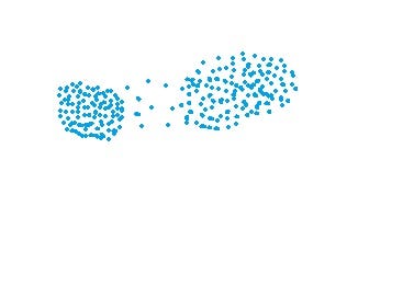
To understand better let’s see a pictorial representation of the Agglomerative Hierarchical clustering Technique. Lets say we have six data points {A,B,C,D,E,F}.

• Step- 1: In the initial step, we calculate the proximity of individual points and consider all the six data points as individual clusters as shown in the image below.

Agglomerative Hierarchical Clustering Technique

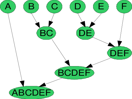
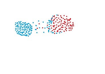
• Step- 2: In step two, similar clusters are merged together and formed as a single cluster. Let’s consider B,C, and D,E are similar clusters that are merged in step two. Now, we’re left with four clusters which are A, BC, DE, F.
• Step- 3: We again calculate the proximity of new clusters and merge the similar clusters to form new clusters A, BC, DEF.
• Step- 4: Calculate the proximity of the new clusters. The clusters DEF and BC are similar and merged together to form a new cluster. We’re now left with two clusters A, BCDEF.
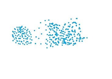
• Step- 5: Finally, all the clusters are merged together and form a single cluster.

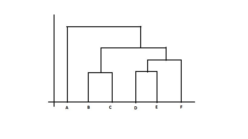
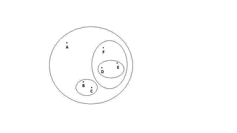
The Hierarchical clustering Technique can be visualized using a Dendrogram.

A Dendrogram is a tree-like diagram that records the sequences of merges or splits.

Dendrogram representation

2. Divisive Hierarchical clustering Technique: Since the Divisive Hierarchical clustering Technique is not much used in the real world, I’ll give a brief of the Divisive Hierarchical clustering Technique.

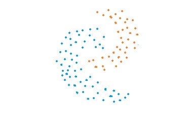
In simple words, we can say that the Divisive Hierarchical clustering is exactly the opposite of the Agglomerative Hierarchical clustering. In Divisive Hierarchical clustering, we consider all the data points as a single cluster and in each iteration, we separate the data points from the cluster which are not similar. Each data point which is separated is considered as an individual cluster. In the end, we’ll be left with n clusters.

As we’re dividing the single clusters into n clusters, it is named as Divisive Hierarchical clustering.

So, we’ve discussed the two types of the Hierarchical clustering Technique.

But wait!! we’re still left with the important part of Hierarchical clustering.

“HOW DO WE CALCULATE THE SIMILARITY BETWEEN TWO CLUSTERS???”

Calculating the similarity between two clusters is important to merge or divide the clusters. There are certain approaches which are used to calculate the similarity between two clusters:

• MIN
• MAX
• Group Average
• Distance Between Centroids
• Ward’s Method
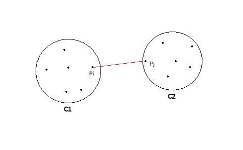
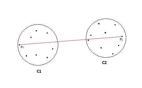
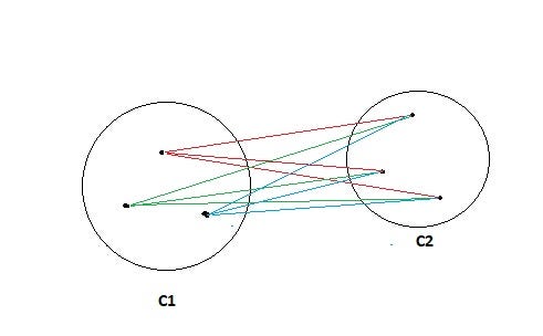
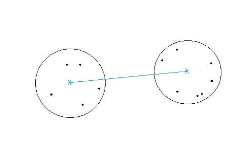
• MIN: Also known as single-linkage algorithm can be defined as the similarity of two clusters C1 and C2 is equal to the minimum of the similarity between points Pi and Pj such that Pi belongs to C1 and Pj belongs to C2.

Mathematically this can be written as,

Sim(C1,C2) = Min Sim(Pi,Pj) such that Pi ∈ C1 & Pj ∈ C2

In simple words, pick the two closest points such that one point lies in cluster one and the other point lies in cluster 2 and takes their similarity and declares it as the similarity between two clusters.

Pros of MIN:

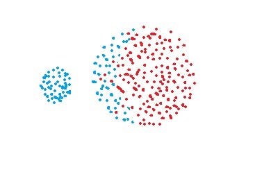
• This approach can separate non-elliptical shapes as long as the gap between the two clusters is not small.

Original data vs Clustered data using MIN approach

Cons of MIN:

• MIN approach cannot separate clusters properly if there is noise between clusters.

Original data vs Clustered data using MIN approach

• MAX: Also known as the complete linkage algorithm, this is exactly opposite to the MIN approach. The similarity of two clusters C1 and C2 is equal to the maximum of the similarity between points Pi and Pj such that Pi belongs to C1 and Pj belongs to C2.

Mathematically this can be written as,

Sim(C1,C2) = Max Sim(Pi,Pj) such that Pi ∈ C1 & Pj ∈ C2

In simple words, pick the two farthest points such that one point lies in cluster one and the other point lies in cluster 2 and takes their similarity and declares it as the similarity between two clusters.

Pros of MAX:

• MAX approach does well in separating clusters if there is noise between clusters.

Original data vs Clustered data using MAX approach

Cons of Max:

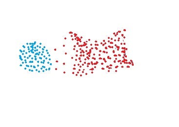
• Max approach is biased towards globular clusters.
• Max approach tends to break large clusters.

Original data vs Clustered data using MAX approach

• Group Average: Take all the pairs of points and compute their similarities and calculate the average of the similarities.

Mathematically this can be written as,

sim(C1,C2) = ∑ sim(Pi, Pj)/|C1|*|C2|

where, Pi ∈ C1 & Pj ∈ C2

Pros of Group Average:

• The group Average approach does well in separating clusters if there is noise between clusters.

Cons of Group Average:

• The group Average approach is biased towards globular clusters.
• Distance between centroids: Compute the centroids of two clusters C1 & C2 and take the similarity between the two centroids as the similarity between two clusters. This is a less popular technique in the real world.

• Ward’s Method: This approach of calculating the similarity between two clusters is exactly the same as Group Average except that Ward’s method calculates the sum of the square of the distances Pi and PJ.

Mathematically this can be written as,

sim(C1,C2) = ∑ (dist(Pi, Pj))²/|C1|*|C2|

Pros of Ward’s method:

• Ward’s method approach also does well in separating clusters if there is noise between clusters.

Cons of Ward’s method:

• Ward’s method approach is also biased towards globular clusters.

Space and Time Complexity of Hierarchical clustering Technique:

Space complexity: The space required for the Hierarchical clustering Technique is very high when the number of data points are high as we need to store the similarity matrix in the RAM. The space complexity is the order of the square of n.

Space complexity = O(n²) where n is the number of data points.

Time complexity: Since we’ve to perform n iterations and in each iteration, we need to update the similarity matrix and restore the matrix, the time complexity is also very high. The time complexity is the order of the cube of n.

Time complexity = O(n³) where n is the number of data points.

Limitations of Hierarchical clustering Technique:

1. There is no mathematical objective for Hierarchical clustering.
2. All the approaches to calculate the similarity between clusters has its own disadvantages.
3. High space and time complexity for Hierarchical clustering. Hence this clustering algorithm cannot be used when we have huge data